<?xml version="1.0" encoding="utf-8"?><feed xmlns="http://www.w3.org/2005/Atom" ><generator uri="https://jekyllrb.com/" version="3.10.0">Jekyll</generator><link href="https://chamoda.com/feed.xml" rel="self" type="application/atom+xml" /><link href="https://chamoda.com/" rel="alternate" type="text/html" /><updated>2026-02-22T13:22:03+00:00</updated><id>https://chamoda.com/feed.xml</id><title type="html">Chamoda Pandithage</title><subtitle>Code, strategy, and first principles thinking.</subtitle><entry><title type="html">Software is no longer a moat</title><link href="https://chamoda.com/software-is-no-longer-a-moat" rel="alternate" type="text/html" title="Software is no longer a moat" /><published>2026-02-21T00:00:00+00:00</published><updated>2026-02-21T00:00:00+00:00</updated><id>https://chamoda.com/software-is-no-longer-a-moat</id><content type="html" xml:base="https://chamoda.com/software-is-no-longer-a-moat"><![CDATA[<p>For decades, software looked like a moat. Building a complex product took years and that friction kept competitors out. But it was almost always the underlying business dynamics that the software enabled, the network effects it accumulated, the proprietary data it generated, the relationships it locked in. The code was just the hard-to-replicate vessel.</p>

<p>Now AI is collapsing that timeline, stripping away the vessel, and forcing a clearer view of what was actually defensible all along.</p>

<p>If software becomes nearly free to build and AI models become commoditized, where does economic value actually get captured?</p>

<h2 id="software-is-no-longer-a-moat">Software is no longer a moat</h2>

<p>No one can build Chrome in a weekend yet, but the amount of human-years it took to write that code are compressing by Nx or more. AI companies know this, so they’re scrambling to build secondary moats: vertically integrated software platforms on top of their models, and user feedback loops that generate proprietary training data.</p>

<p>Software will probably never be truly “free”, there will always be human product management, design decisions, and coordination involved. But the cost curve is dropping fast enough that software alone can no longer protect a business. The companies that thought they were selling software were often really selling something else. AI makes that distinction impossible to ignore.</p>

<h2 id="data-isnt-the-best-moat-either">Data isn’t the best moat either</h2>

<p>As Ilya Sutskever put it: “We’ve achieved peak data and there’ll be no more”, comparing human-generated content to a finite resource like oil.</p>

<p>And even this scarcity might not matter. Synthetic data is proving nearly as good as real data, sometimes better for edge cases. The data moat is eroding faster than most expected.</p>

<h2 id="what-moats-still-exist">What moats still exist?</h2>

<p>In a world where both AI models and software are commoditized, value gets captured elsewhere</p>

<p><strong>Compute</strong> - Physical infrastructure is hard to replicate. In the short run, compute is scarce and the supply chain for creating more is undersupplied. Cloud providers like GCP, Azure, and AWS will have serious moats as long as GPU capacity remains a genuinely scarce resource.</p>

<p><strong>Human relationships</strong> - Partnerships, contracts, brand recognition, and social networks are hard to replace even if the underlying software becomes trivial to rebuild.</p>

<p><strong>Capital</strong> - Cash in the bank to weather competition and outlast races to the bottom.</p>

<p><strong>Proprietary data</strong> - Not scraped or synthesized data, but data that only you can generate: operational data, customer behavior, private records.</p>

<p><strong>Team</strong> - Rare talent that competitors can’t easily hire away.</p>

<p><strong>Exclusive rights</strong> - Patents, trademarks, copyrights, regulatory licenses.</p>

<p><strong>Network effects</strong> - Value that scales with users in ways that are hard to bootstrap from scratch.</p>

<h2 id="the-weakest-position">The weakest position</h2>

<p>Companies with the weakest moats right now are probably pure software companies. SaaS businesses and AI model creators who bet that the software or model itself was the defensible asset. It wasn’t. The question for all of them is: what’s the real moat underneath?</p>

<h2 id="the-strongest-moats">The strongest moats</h2>

<p>So what will have the strongest moats in an AI-commoditized world?</p>

<p><strong>Energy and logistics</strong> - Companies that can produce and transport energy at scale, with the right land and water rights. AI runs on electricity and cooling; whoever controls those inputs sits at the foundation of the whole stack.</p>

<p><strong>Geography-locked compute</strong> - Data centers built next to scarce energy and water sources, where location itself becomes the moat.</p>

<p><strong>Deep relationships</strong> - Companies like Meta or ByteDance with billions of users and entrenched network effects. Government contractors locked into long, custom contracts with institutional relationships that take decades to build and are nearly impossible to displace, regardless of what software can do.</p>

<p>The set of things worth building just got a lot bigger. The moats around those things just got a lot smaller.</p>]]></content><author><name></name></author><summary type="html"><![CDATA[If software becomes nearly free to build and AI models become commoditized, where does economic value actually get captured?]]></summary></entry><entry><title type="html">Public-key cryptography explained</title><link href="https://chamoda.com/public-key-cryptography-explained" rel="alternate" type="text/html" title="Public-key cryptography explained" /><published>2017-12-13T00:00:00+00:00</published><updated>2017-12-13T00:00:00+00:00</updated><id>https://chamoda.com/public-key-cryptography-explained</id><content type="html" xml:base="https://chamoda.com/public-key-cryptography-explained"><![CDATA[<p>Public-key cryptography is one of the most used cryptosystems today. It refers to any system that uses a key pair, one for encrypting data and another one for decrypting data. If data is encrypted using a key, the other key is used to decrypt it. This seems pretty magical at first, but by the end of this blog post you will understand how this works. In this blog post I’ll start with an analogy to understand what the purpose of using two key pairs is. Then I’ll explain the mathematical concepts behind the algorithm. Then I’ll implement a toy algorithm to understand it further (But never design your own crypto algorithms). Next I’ll explain some <code class="language-plaintext highlighter-rouge">openssl</code> commands to generate RSA public and private keys which you can use in real world applications.</p>

<h2 id="lets-start-with-an-analogy">Let’s start with an analogy</h2>

<p>Suppose you are at home and need to send your passbook to the bank. You have to send this by a bad courier service, in fact they always try to inspect and spy on what’s inside every package. So you buy a locker box with two identical keys. You keep one to yourself and send the other one to the bank. You can’t send the key with the package because the courier service will open the locker box and inspect. You can’t send it separately because this bad courier always makes copies of the keys they deliver in hopes of trying them out on future deliveries. So you walk into the bank yourself to deliver the key to the bank. Now you go home and put the passbook inside the locker box and lock it with your identical key and send it via the bad courier. They deliver the box hopelessly without being able to see what’s inside. It was inefficient, you had to visit the bank yourself first. But can we do better?</p>

<p>This time the bank buys a new kind of locker for this purpose. The new locker box has two keys, one for locking the box (public key), another one for unlocking (private key). The key used to lock can’t be used to unlock the box. The key used to unlock can’t be used to lock the box. The bank sends over the locker box to you along with the locking key (public key). As usual the bad courier makes a copy of the key in hopes of future endeavors. Now you put the passbook inside the box and lock it with your locking key (public key). You keep the key and send the box. The courier tries to unlock the box using the key they have copied, but no luck. It can only be unlocked using the unlocking key (private key) only owned by the bank.</p>

<p>The modern Internet is like the bad courier, filled with hackers inspecting unencrypted packets. We need something similar to the second paragraph to secure Internet communication.</p>

<p>The first paragraph is an analogy of symmetric encryption. The second paragraph discusses asymmetric encryption, which is the category public encryption belongs to. But how could we design such a lock digitally?</p>

<h2 id="the-underlying-mathematics">The underlying mathematics</h2>

<p>We can write our encryption function as \(C = E(M)\) where \(M\) is the message we want to encrypt, \(E\) is the function that does the encryption and \(C\) is the encrypted message. Decryption is \(M = D(C)\). Let’s define our functions.</p>

\[E(M) = M^e \bmod n\]

\[D(C) = C^d \bmod n\]

<p>\(e\) and \(d\) are public and private keys respectively. \(n\) is a large number which is a multiple of two large prime numbers. \(\bmod\) means the modulo operation. Most programming languages represent this by <code class="language-plaintext highlighter-rouge">%</code> symbol. Given two positive numbers \(a\) and \(n\) result of \(a \bmod n\) is the reminder when \(a\) divides by \(n\). For example \(7 \bmod 3 = 1\) because when \(7\) divides by \(3\) remainder is \(1\). We could write above equations in another way using modular arithmetic syntax.</p>

\[E(M) \equiv M^e \pmod{n}\]

\[D(C) \equiv C^d \pmod{n}\]

<p>If \(a \equiv b \pmod{n}\) then \(a\) and \(b\) have a congruence relationship. That means \(a - b\) is divisible by \(n\) and \(a \bmod n\) and \(b \bmod n\) both have the same remainder.</p>

<p>Now we can write the following congruence relation. This relationship must be true for encryption and decryption to work properly. \(D(E(M))\) must always return original \(M\) back.</p>

\[M \equiv D(E(M)) \equiv (M^e)^d \pmod{n}\]

<p>Now we need to find a relationship between \(e\) and \(d\) such that \(D(E(M))\) holds true. To move forward we need another equation. For that we are going to start with Fermat’s little theorem from number theory. The theorem states the following</p>

\[a^p \equiv a \pmod{p}\]

<p>If \(p\) is a prime number and \(a\) is any integer, \(a^p - a\) is an integer multiple of \(p\). We can also write this as</p>

\[a \times a^{p - 1} \equiv a \times 1 \pmod{p}\]

<p>Removing \(a\) from both sides we get</p>

\[a^{p - 1} \equiv 1 \pmod{p}\]

<p>Now let’s look at a function called Euler’s totient function. In number theory Euler’s totient function counts the number of positive integers for a given integer \(n\) that are relatively prime to \(n\). Relative primes are numbers that don’t have common divisors other than \(1\). If \(a\) and \(b\) are relatively prime then we can write that the greatest common divisor is \(1\). We usually write this as \(gcd(a, b) = 1\). For example \(10\) and \(7\) are relatively prime because \(gcd(10, 7) = 1\). Now to the totient function, notice that if \(n\) is a prime all the positive integers less than \(n\) are relatively prime to \(n\). We can write this as</p>

\[\phi(n) = n - 1\]

<p>So what does it have to do with our previous equations? Now we can write something like this using Euler’s totient function.</p>

\[M^{\phi(n)} \equiv 1 \pmod{n}\]

<p>Now we are going to prepare the above equations to match \(M^{ed} \equiv M \pmod{n}\) which is similar to \(M \equiv D(E(M)) \equiv (M^e)^d \pmod{n}\) with some reordering. As the first step of the preparation, take the power \(k\) on both sides</p>

\[M^{k\phi(n)} \equiv 1^k \pmod{n}\]

<p>Since \(1^k\) is \(1\)</p>

\[M^{k\phi(n)} \equiv 1 \pmod{n}\]

<p>Now Let’s multiply both sides by \(M\)</p>

\[M \times M^{k\phi(n)} \equiv M \times 1 \pmod{n}\]

\[M^{k\phi(n) + 1} \equiv M \pmod{n}\]

<p>Now we also have the following equation</p>

\[M^{ed} \equiv M \pmod{n}\]

<p>Did you notice the similarity in the right side of the two equations? Now we can write</p>

\[k\phi(n) + 1 = ed\]

<p>Now this is exactly the following by the definition of modular arithmetic syntax.</p>

\[ed \equiv 1 \pmod{\phi(n)}\]

<p>We can expand \(\phi(n)\) further because \(n\) is a multiple of two prime numbers.</p>

\[n = p \times q\]

\[\phi(n) = \phi(p) \times \phi(q)\]

\[\phi(n) = (p - 1) \times (q - 1)\]

<p>So we can write</p>

\[ed \equiv 1 \pmod{(p -1 )(q - 1)}\]

<p>Now choose a random private key \(d\) such that \(1 &lt; d &lt; \phi(n)\) and \(gcd(d, \phi(n)) = 1\) (which means they need to be relatively prime). Now we can find \(e\) using the modular inverse algorithm.</p>

<p>Now that we have found keys \(e\) and \(d\) we can use them to encrypt and decrypt messages. In the next section I will give a numeric example which will clear up most of the details.</p>

<h2 id="numerical-example">Numerical example</h2>

<p>Let’s choose two prime numbers \(p\) and \(q\). We choose small values to make calculations easier but in practice the RSA algorithm uses very large prime numbers.</p>

\[p = 3\]

\[q = 11\]

\[n = p \times q = 3 \times 11 = 33\]

<p>And let’s calculate the Euler’s totient function</p>

\[\phi(n) = (p - 1)(q - 1) = 2 \times 10 = 20\]

<p>Now we choose \(d\) such that it’s relatively prime to \(\phi(n)\). Let’s say</p>

\[d = 7\]

<p>Now compute \(e\) such that</p>

\[d \times e \bmod \phi(n) = 1\]

\[7 \times e \bmod 20 = 1\]

<p>If \(e = 3\) then \(7 \times 3 \bmod 20 = 1\) satisfies the equation.</p>

<p>Now the private key is \(d = (7, 33)\) and the public key is \(e = (3, 33)\). Now let’s encrypt some number \(M = 2\) using the public key. Of course if you need to encrypt characters you must convert them to integers first.</p>

\[C = M^e \bmod n\]

\[C = 2^3 \bmod 33\]

\[C = 8\]

<p>Now let’s decrypt \(C\) using the private key.</p>

\[M = C^d \bmod n\]

\[M = 8^7 \bmod 33\]

\[M = 2\]

<p>It works :). I’ve implemented this as a toy algorithm using python. Never implement your own cryptography algorithms though, for use in production environments.</p>

<div class="language-python highlighter-rouge"><div class="highlight"><pre class="highlight"><code><span class="kn">from</span> <span class="nn">__future__</span> <span class="kn">import</span> <span class="n">division</span>
<span class="kn">from</span> <span class="nn">Crypto.Util</span> <span class="kn">import</span> <span class="n">number</span>
<span class="kn">import</span> <span class="nn">os</span>
<span class="kn">from</span> <span class="nn">fractions</span> <span class="kn">import</span> <span class="n">gcd</span>
</code></pre></div></div>

<p><code class="language-plaintext highlighter-rouge">from Crypto.Util import number</code> for generating random primes.</p>

<div class="language-python highlighter-rouge"><div class="highlight"><pre class="highlight"><code><span class="k">class</span> <span class="nc">RSA</span><span class="p">:</span>    
    <span class="n">p</span> <span class="o">=</span> <span class="n">q</span> <span class="o">=</span> <span class="n">n</span> <span class="o">=</span> <span class="n">d</span> <span class="o">=</span> <span class="n">e</span> <span class="o">=</span> <span class="n">pi_n</span> <span class="o">=</span> <span class="mi">0</span>
    
    <span class="k">def</span> <span class="nf">__init__</span><span class="p">(</span><span class="bp">self</span><span class="p">):</span>        
        <span class="bp">self</span><span class="p">.</span><span class="n">generate</span><span class="p">()</span>
        
    <span class="k">def</span> <span class="nf">generate</span><span class="p">(</span><span class="bp">self</span><span class="p">):</span>        
        <span class="bp">self</span><span class="p">.</span><span class="n">p</span> <span class="o">=</span> <span class="n">number</span><span class="p">.</span><span class="n">getPrime</span><span class="p">(</span><span class="mi">10</span><span class="p">,</span> <span class="n">os</span><span class="p">.</span><span class="n">urandom</span><span class="p">)</span>
        <span class="bp">self</span><span class="p">.</span><span class="n">q</span> <span class="o">=</span> <span class="n">number</span><span class="p">.</span><span class="n">getPrime</span><span class="p">(</span><span class="mi">10</span><span class="p">,</span> <span class="n">os</span><span class="p">.</span><span class="n">urandom</span><span class="p">)</span>        
        <span class="bp">self</span><span class="p">.</span><span class="n">n</span> <span class="o">=</span> <span class="bp">self</span><span class="p">.</span><span class="n">p</span> <span class="o">*</span> <span class="bp">self</span><span class="p">.</span><span class="n">q</span>        
        <span class="bp">self</span><span class="p">.</span><span class="n">pi_n</span> <span class="o">=</span> <span class="p">(</span><span class="bp">self</span><span class="p">.</span><span class="n">p</span> <span class="o">-</span> <span class="mi">1</span><span class="p">)</span> <span class="o">*</span> <span class="p">(</span><span class="bp">self</span><span class="p">.</span><span class="n">q</span> <span class="o">-</span> <span class="mi">1</span><span class="p">)</span>        
        <span class="bp">self</span><span class="p">.</span><span class="n">d</span> <span class="o">=</span> <span class="bp">self</span><span class="p">.</span><span class="n">choose_d</span><span class="p">()</span>        
        <span class="bp">self</span><span class="p">.</span><span class="n">e</span> <span class="o">=</span> <span class="bp">self</span><span class="p">.</span><span class="n">choose_e</span><span class="p">()</span>
        
    <span class="k">def</span> <span class="nf">choose_d</span><span class="p">(</span><span class="bp">self</span><span class="p">):</span>        
        <span class="bp">self</span><span class="p">.</span><span class="n">d</span> <span class="o">=</span> <span class="bp">self</span><span class="p">.</span><span class="n">find_a_coprime</span><span class="p">(</span><span class="bp">self</span><span class="p">.</span><span class="n">pi_n</span><span class="p">)</span>        
        <span class="k">return</span> <span class="bp">self</span><span class="p">.</span><span class="n">d</span>
                    
    <span class="k">def</span> <span class="nf">find_a_coprime</span><span class="p">(</span><span class="bp">self</span><span class="p">,</span> <span class="n">a</span><span class="p">):</span>        
        <span class="k">for</span> <span class="n">i</span> <span class="ow">in</span> <span class="nb">range</span><span class="p">(</span><span class="mi">2</span><span class="p">,</span> <span class="n">a</span><span class="p">):</span>            
            <span class="k">if</span> <span class="n">gcd</span><span class="p">(</span><span class="n">i</span><span class="p">,</span> <span class="n">a</span><span class="p">)</span> <span class="o">==</span> <span class="mi">1</span><span class="p">:</span>                
                <span class="k">return</span> <span class="n">i</span>
            
    <span class="k">def</span> <span class="nf">choose_e</span><span class="p">(</span><span class="bp">self</span><span class="p">):</span>        
        <span class="k">for</span> <span class="n">i</span> <span class="ow">in</span> <span class="nb">range</span><span class="p">(</span><span class="bp">self</span><span class="p">.</span><span class="n">n</span><span class="p">):</span>            
            <span class="k">if</span> <span class="p">(</span><span class="n">i</span> <span class="o">*</span> <span class="bp">self</span><span class="p">.</span><span class="n">d</span><span class="p">)</span> <span class="o">%</span> <span class="bp">self</span><span class="p">.</span><span class="n">pi_n</span> <span class="o">==</span> <span class="mi">1</span><span class="p">:</span>                
                <span class="k">return</span> <span class="n">i</span>
    
    <span class="k">def</span> <span class="nf">public_key</span><span class="p">(</span><span class="bp">self</span><span class="p">):</span>        
        <span class="k">return</span> <span class="p">(</span><span class="bp">self</span><span class="p">.</span><span class="n">e</span><span class="p">,</span> <span class="bp">self</span><span class="p">.</span><span class="n">n</span><span class="p">)</span>
    
    <span class="k">def</span> <span class="nf">private_key</span><span class="p">(</span><span class="bp">self</span><span class="p">):</span>        
        <span class="k">return</span> <span class="p">(</span><span class="bp">self</span><span class="p">.</span><span class="n">d</span><span class="p">,</span> <span class="bp">self</span><span class="p">.</span><span class="n">n</span><span class="p">)</span>
    
    <span class="k">def</span> <span class="nf">encrypt</span><span class="p">(</span><span class="bp">self</span><span class="p">,</span> <span class="n">m</span><span class="p">,</span> <span class="n">key</span><span class="p">):</span>        
        <span class="k">return</span> <span class="nb">pow</span><span class="p">(</span><span class="n">m</span><span class="p">,</span> <span class="n">key</span><span class="p">[</span><span class="mi">0</span><span class="p">])</span> <span class="o">%</span> <span class="n">key</span><span class="p">[</span><span class="mi">1</span><span class="p">]</span>
    
    <span class="k">def</span> <span class="nf">decrypt</span><span class="p">(</span><span class="bp">self</span><span class="p">,</span> <span class="n">c</span><span class="p">,</span> <span class="n">key</span><span class="p">):</span>        
        <span class="k">return</span> <span class="nb">pow</span><span class="p">(</span><span class="n">c</span><span class="p">,</span> <span class="n">key</span><span class="p">[</span><span class="mi">0</span><span class="p">])</span> <span class="o">%</span> <span class="n">key</span><span class="p">[</span><span class="mi">1</span><span class="p">]</span>
</code></pre></div></div>

<p>Now we can create <code class="language-plaintext highlighter-rouge">RSA</code> class</p>

<div class="language-python highlighter-rouge"><div class="highlight"><pre class="highlight"><code><span class="n">rsa</span> <span class="o">=</span> <span class="n">RSA</span><span class="p">()</span>
</code></pre></div></div>

<p>Following should output <code class="language-plaintext highlighter-rouge">99</code> if our algorithm works and it does :)</p>

<div class="language-python highlighter-rouge"><div class="highlight"><pre class="highlight"><code><span class="n">rsa</span><span class="p">.</span><span class="n">decrypt</span><span class="p">(</span><span class="n">rsa</span><span class="p">.</span><span class="n">encrypt</span><span class="p">(</span><span class="mi">99</span><span class="p">,</span> <span class="n">rsa</span><span class="p">.</span><span class="n">public_key</span><span class="p">()),</span> <span class="n">rsa</span><span class="p">.</span><span class="n">private_key</span><span class="p">())</span>
</code></pre></div></div>

<h2 id="how-is-it-secure">How is it secure</h2>

<p>The whole security of public key encryption depends on the fact that given a public key no one should be able to generate the private key from that public key. Remember \(ed \equiv 1 \pmod{\phi(n)}\)? So, to calculate d from e an attacker needs to know \(\phi(n)\). But the only way to calculate that is \((p - 1)(q - 1)\). Only the key generator knows \(p\) and \(q\). When \(p\) and \(q\) are large enough no one can calculate (yet!) \(p\) and \(q\) from \(n\). The whole cryptosystem depends on this assumption.</p>

<h2 id="practical-usage">Practical usage</h2>

<p>Public key cryptography is used everywhere. HTTPS runs on public key cryptography (not only RSA but it plays a huge role). If you need to use public key cryptography for your own application you can use openssl. openssl is a full featured toolkit which can generate RSA keys among lots of other things. To generate a key pair type the following in the command line (assuming you are on a UNIX based system)</p>

<div class="language-plaintext highlighter-rouge"><div class="highlight"><pre class="highlight"><code>openssl genpkey -algorithm RSA -out private_key.pem -pkeyopt rsa_keygen_bits:2048
</code></pre></div></div>

<p>You will generate a <code class="language-plaintext highlighter-rouge">private_key.pem</code> file from the above command. In this key there is lots of information encoded so that it can be used to extract the public key.</p>

<div class="language-plaintext highlighter-rouge"><div class="highlight"><pre class="highlight"><code>openssl rsa -pubout -in private_key.pem -out public_key.pem
</code></pre></div></div>

<p><code class="language-plaintext highlighter-rouge">public_key.pem</code> only contains details to encrypt or decrypt something so it can be shared. But you should never share your <code class="language-plaintext highlighter-rouge">private_key.pem</code></p>

<p>Now let’s encrypt some data using public key.</p>

<div class="language-plaintext highlighter-rouge"><div class="highlight"><pre class="highlight"><code>echo "reqviescat in constantia, ergo, repræsentatio cvpidi avctoris religionis" &gt; key.bin
</code></pre></div></div>

<div class="language-plaintext highlighter-rouge"><div class="highlight"><pre class="highlight"><code>openssl rsautl -encrypt -inkey public_key.pem -pubin -in key.bin -out key.bin.enc
</code></pre></div></div>

<p>Encrypted data is written to <code class="language-plaintext highlighter-rouge">key.bin.enc</code>. Now let’s decrypt it again</p>

<div class="language-plaintext highlighter-rouge"><div class="highlight"><pre class="highlight"><code>openssl rsautl -decrypt -inkey private_key.pem -in key.bin.enc -out key.bin
</code></pre></div></div>

<p>If you open the <code class="language-plaintext highlighter-rouge">key.bin</code> file you can see that the same data is there.</p>

<h2 id="additional-resources">Additional resources</h2>

<ul>
  <li>Toy RSA Algorithm - <a href="https://github.com/chamoda/rsa-algorithm">GitHub</a></li>
  <li>Original RSA Paper - <a href="https://people.csail.mit.edu/rivest/Rsapaper.pdf">A Method for Obtaining Digital Signatures and Public-Key Cryptosystems</a></li>
  <li>Modular Arithmetic - <a href="https://en.wikipedia.org/wiki/Modular_arithmetic">Wikipedia</a></li>
  <li>Fermat’s Little Theorem - <a href="https://en.wikipedia.org/wiki/Fermat%27s_little_theorem">Wikipedia</a></li>
  <li>Coprime integers - <a href="https://en.wikipedia.org/wiki/Coprime_integers">Wikipedia</a></li>
  <li>Euler’s totient function - <a href="https://en.wikipedia.org/wiki/Euler%27s_totient_function">Wikipedia</a></li>
  <li>Modular multiplicative inverse - <a href="https://en.wikipedia.org/wiki/Modular_multiplicative_inverse">Wikipedia</a></li>
</ul>]]></content><author><name></name></author><summary type="html"><![CDATA[Understand how public-key cryptography works with RSA encryption. Learn the mathematical concepts, see a toy implementation, and get practical OpenSSL commands for real-world use.]]></summary></entry><entry><title type="html">Real time face detection using OpenCV and Python</title><link href="https://chamoda.com/realtime-face-detection-using-opencv-and-python" rel="alternate" type="text/html" title="Real time face detection using OpenCV and Python" /><published>2017-11-18T00:00:00+00:00</published><updated>2017-11-18T00:00:00+00:00</updated><id>https://chamoda.com/realtime-face-detection-using-opencv-and-python</id><content type="html" xml:base="https://chamoda.com/realtime-face-detection-using-opencv-and-python"><![CDATA[<p>Detection is an important application in computer vision. In this post I’m going to detail how to do real time face detection using the Viola Jones Algorithm introduced in the paper <a href="http://citeseerx.ist.psu.edu/viewdoc/summary?doi=10.1.1.10.6807">Rapid object detection using a boosted cascade of simple features (2001)</a>. Mind the word detection, we are not going to recognize, meaning which one the face belongs to. This is merely detection that there is a face in a given image. We are going to use <a href="https://opencv.org">OpenCV</a> (Open Source Computer Vision Library). OpenCV is written in C++ but there are interfaces for other languages so we will use, preferably python.</p>

<h2 id="installation">Installation</h2>

<p>Instructions are for OSX. Steps are as follows</p>

<ul>
  <li>First install <a href="https://www.anaconda.com/download/">Anaconda</a>.</li>
  <li>Then create python 3 virtual environment with <code class="language-plaintext highlighter-rouge">conda create -n py3 python=3.6</code>.</li>
  <li>Then type <code class="language-plaintext highlighter-rouge">source activate py3</code> which will activate python 3 environment.</li>
  <li>Now install opencv with <code class="language-plaintext highlighter-rouge">conda install -c conda-forge opencv</code>.</li>
  <li>Check the installation with <code class="language-plaintext highlighter-rouge">echo -e "import cv2; print(cv2.__version__)" | python</code> command. It should output <code class="language-plaintext highlighter-rouge">3.3.0</code></li>
  <li>Make sure your system has <code class="language-plaintext highlighter-rouge">ffmpeg</code> installed which is required for reading a video stream from video formats like <code class="language-plaintext highlighter-rouge">mp4, mkv</code>. Using brew you can install ffmpeg with one command <code class="language-plaintext highlighter-rouge">brew install ffmpeg</code></li>
</ul>

<h2 id="time-for-action">Time for action</h2>

<p>Let’s do a quick implementation.</p>

<div class="language-python highlighter-rouge"><div class="highlight"><pre class="highlight"><code><span class="kn">import</span> <span class="nn">cv2</span>

<span class="n">cap</span> <span class="o">=</span> <span class="n">cv2</span><span class="p">.</span><span class="n">VideoCapture</span><span class="p">(</span><span class="s">"input.mp4"</span><span class="p">)</span>
<span class="n">face_cascade</span> <span class="o">=</span> <span class="n">cv2</span><span class="p">.</span><span class="n">CascadeClassifier</span><span class="p">(</span><span class="s">'haarcascade_frontalface_default.xml'</span><span class="p">)</span>

<span class="k">while</span><span class="p">(</span><span class="bp">True</span><span class="p">):</span>
    <span class="n">ret</span><span class="p">,</span> <span class="n">frame</span> <span class="o">=</span> <span class="n">cap</span><span class="p">.</span><span class="n">read</span><span class="p">()</span>
    <span class="n">gray</span> <span class="o">=</span> <span class="n">cv2</span><span class="p">.</span><span class="n">cvtColor</span><span class="p">(</span><span class="n">frame</span><span class="p">,</span> <span class="n">cv2</span><span class="p">.</span><span class="n">COLOR_BGR2GRAY</span><span class="p">)</span>
    <span class="n">faces</span> <span class="o">=</span> <span class="n">face_cascade</span><span class="p">.</span><span class="n">detectMultiScale</span><span class="p">(</span><span class="n">gray</span><span class="p">,</span> <span class="mf">1.3</span><span class="p">,</span> <span class="mi">5</span><span class="p">)</span> 
    
    <span class="k">for</span> <span class="p">(</span><span class="n">x</span><span class="p">,</span><span class="n">y</span><span class="p">,</span><span class="n">w</span><span class="p">,</span><span class="n">h</span><span class="p">)</span> <span class="ow">in</span> <span class="n">faces</span><span class="p">:</span>
      <span class="n">cv2</span><span class="p">.</span><span class="n">rectangle</span><span class="p">(</span><span class="n">frame</span><span class="p">,</span> <span class="p">(</span><span class="n">x</span><span class="p">,</span> <span class="n">y</span><span class="p">),</span> <span class="p">(</span><span class="n">x</span><span class="o">+</span><span class="n">w</span><span class="p">,</span> <span class="n">y</span><span class="o">+</span><span class="n">h</span><span class="p">),</span> <span class="p">(</span><span class="mi">0</span> <span class="p">,</span> <span class="mi">0</span><span class="p">,</span> <span class="mi">255</span><span class="p">),</span> <span class="mi">2</span><span class="p">)</span>
    
    <span class="n">cv2</span><span class="p">.</span><span class="n">imshow</span><span class="p">(</span><span class="s">'frame'</span><span class="p">,</span> <span class="n">frame</span><span class="p">)</span>

    <span class="k">if</span> <span class="n">cv2</span><span class="p">.</span><span class="n">waitKey</span><span class="p">(</span><span class="mi">1</span><span class="p">)</span> <span class="o">&amp;</span> <span class="mh">0xFF</span> <span class="o">==</span> <span class="nb">ord</span><span class="p">(</span><span class="s">'q'</span><span class="p">):</span>        
        <span class="k">break</span>

<span class="n">cap</span><span class="p">.</span><span class="n">release</span><span class="p">()</span>
<span class="n">cv2</span><span class="p">.</span><span class="n">destroyAllWindows</span><span class="p">()</span>
</code></pre></div></div>

<p>
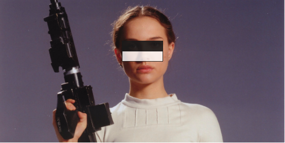
We are going to read a video file frame by frame, applying the Viola Jones algorithm with trained parameters then apply a rectangle layer if a face is found, displaying the modified output frame by frame.</p>

<p><code class="language-plaintext highlighter-rouge">cap = cv2.VideoCapture("input.mp4")</code> imports the video. You can also use a web cam instead of video, just pass <code class="language-plaintext highlighter-rouge">0</code> as parameter like <code class="language-plaintext highlighter-rouge">cap = cv2.VideoCapture(0)</code>.</p>

<p>Next we are going to load the trained model. <code class="language-plaintext highlighter-rouge">haarcascade_frontalface_default.xml</code> is a model already trained using lots of faces and non-faces and lots of computing power. Training good models sometimes takes days not hours. Thankfully the above model is trained by Intel using lots of data. The model we are using here comes with the installation of OpenCV. Generally you can find those models at your <code class="language-plaintext highlighter-rouge">opencv-installation-directory/share/OpenCV/haarcascades</code> but this could differ depending on your OS and installation method.</p>

<p>Next in the <code class="language-plaintext highlighter-rouge">while</code> loop we are reading frame by frame. Then get the given frame and convert it into grayscale.</p>

<div class="language-python highlighter-rouge"><div class="highlight"><pre class="highlight"><code><span class="n">gray</span> <span class="o">=</span> <span class="n">cv2</span><span class="p">.</span><span class="n">cvtColor</span><span class="p">(</span><span class="n">frame</span><span class="p">,</span> <span class="n">cv2</span><span class="p">.</span><span class="n">COLOR_BGR2GRAY</span><span class="p">)</span>
</code></pre></div></div>

<p>A frame is an array of 3 matrices where each matrix is for the respective color blue, green, red. Did you notice the reversed order? In OpenCV the default representation is BGR not RGB. In the above step we are converting it to a grayscale image. <code class="language-plaintext highlighter-rouge">gray</code> is a single matrix now.</p>

<div class="language-python highlighter-rouge"><div class="highlight"><pre class="highlight"><code><span class="n">faces</span> <span class="o">=</span> <span class="n">face_cascade</span><span class="p">.</span><span class="n">detectMultiScale</span><span class="p">(</span><span class="n">gray</span><span class="p">,</span> <span class="mf">1.3</span><span class="p">,</span> <span class="mi">5</span><span class="p">)</span> 
</code></pre></div></div>

<p><code class="language-plaintext highlighter-rouge">detectMultiScale</code> function detects faces and returns an array of position coordinates and sizes. The second parameter is <code class="language-plaintext highlighter-rouge">scaleFactor</code>. To reduce true negatives you must use a value near to zero. Basically the algorithm can only detect its trained size usually around 20x20 pixels. To detect large objects the area gets scaled by <code class="language-plaintext highlighter-rouge">scaleFactor</code>. If <code class="language-plaintext highlighter-rouge">scaleFactor</code> is \(1.05\) the scaled block size would equal to \(20 \times 1.05 = 21\). If <code class="language-plaintext highlighter-rouge">scaleFactor</code> is equal to 1.3 in the above image the scaled block size is \(20 \times 1.3 = 26\) so you may miss some pixels, and thus some faces. The trade-off is accuracy vs performance.</p>

<p>The 3rd parameter is <code class="language-plaintext highlighter-rouge">minNeighbors</code>. It defines how many neighbor rectangles should be identified to retain it. Higher value means fewer false positives.</p>

<p>Next we draw red rectangles if faces are detected. Notice how we passed the red color in BGR format <code class="language-plaintext highlighter-rouge">(0 , 0, 255)</code>.</p>

<div class="language-python highlighter-rouge"><div class="highlight"><pre class="highlight"><code><span class="k">for</span> <span class="p">(</span><span class="n">x</span><span class="p">,</span><span class="n">y</span><span class="p">,</span><span class="n">w</span><span class="p">,</span><span class="n">h</span><span class="p">)</span> <span class="ow">in</span> <span class="n">faces</span><span class="p">:</span>
      <span class="n">cv2</span><span class="p">.</span><span class="n">rectangle</span><span class="p">(</span><span class="n">frame</span><span class="p">,</span> <span class="p">(</span><span class="n">x</span><span class="p">,</span> <span class="n">y</span><span class="p">),</span> <span class="p">(</span><span class="n">x</span><span class="o">+</span><span class="n">w</span><span class="p">,</span> <span class="n">y</span><span class="o">+</span><span class="n">h</span><span class="p">),</span> <span class="p">(</span><span class="mi">0</span> <span class="p">,</span> <span class="mi">0</span><span class="p">,</span> <span class="mi">255</span><span class="p">),</span> <span class="mi">2</span><span class="p">)</span>
</code></pre></div></div>

<p>Next we are writing to a window frame by frame. If you press the key <code class="language-plaintext highlighter-rouge">q</code> the loop will break and the video will stop. I’ve created a quick video from the output here. Notice how it detects only frontal faces because the model is trained for frontal faces.</p>

<iframe width="100%" height="450" src="https://www.youtube.com/embed/eAJwY8fQvXs" frameborder="0" allowfullscreen=""></iframe>

<h2 id="how-it-works">How it works</h2>

<p>The Viola Jones algorithm is a machine learning algorithm developed by Paul Viola and Michael Jones in 2001. It was designed to be very fast, even fast enough to be possible in embedded systems. We can break it down into 4 parts</p>

<ul>
  <li>Haar like features</li>
  <li>Integral image</li>
  <li>AdaBoost (Adaptive Boosting)</li>
  <li>Cascading</li>
</ul>

<h2 id="haar-like-features">Haar like features</h2>

<p>Haar-like features, named after the Hungarian mathematician Alfred Haar, are a way of identifying features in an image in a more abstract way.</p>

<p><img src="https://chamoda.com/assets/posts/realtime-face-detection-using-opencv-and-python/haar.png" alt="Haar" /></p>

<p>
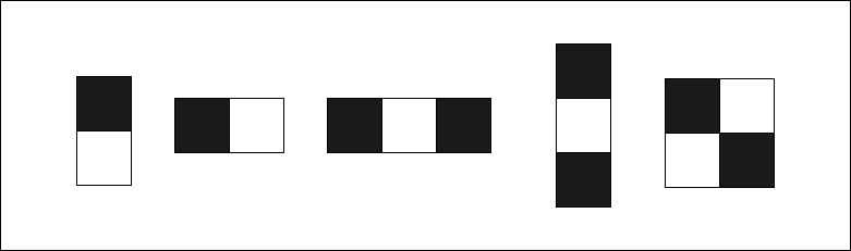
To calculate a feature following equation is used.</p>

\[Value = \text{(Sum of pixels in black area)} - \text{(Sum of pixels in white area)}\]

<p>In the case of face detection the following feature will give a higher value in the positioned area, which defines a feature.</p>

<p><img src="https://chamoda.com/assets/posts/realtime-face-detection-using-opencv-and-python/face.png" alt="Face" /></p>

<p>Eye areas are generally darker than the area under the eye, so \(\text{(Black area - White area)}\) will give a higher value. And that defines a single feature.</p>

<h2 id="integral-image">Integral image</h2>

<p>Integral image is a way to calculate rectangle features quickly</p>

\[ii(x, y) = \sum_{x{'} \le x, y{'} \le y} i(x', y')\]

<p>Every position is the sum of the top and left values. Note this code is written for clarity, there are more efficient ways to write this. In this case you will be feeding a normalized image to the function. The purpose of normalizing first is to get rid of lighting effects.</p>

<div class="language-python highlighter-rouge"><div class="highlight"><pre class="highlight"><code><span class="k">def</span> <span class="nf">my_integral_image</span><span class="p">(</span><span class="n">img</span><span class="p">):</span>
    
    <span class="n">integral_img</span> <span class="o">=</span> <span class="n">np</span><span class="p">.</span><span class="n">zeros</span><span class="p">(</span><span class="n">img</span><span class="p">.</span><span class="n">shape</span><span class="p">)</span>
    <span class="k">for</span> <span class="n">x</span> <span class="ow">in</span> <span class="nb">range</span><span class="p">(</span><span class="n">img</span><span class="p">.</span><span class="n">shape</span><span class="p">[</span><span class="mi">1</span><span class="p">]):</span>
        <span class="k">for</span> <span class="n">y</span> <span class="ow">in</span> <span class="nb">range</span><span class="p">(</span><span class="n">img</span><span class="p">.</span><span class="n">shape</span><span class="p">[</span><span class="mi">0</span><span class="p">]):</span>
            <span class="k">for</span> <span class="n">i</span> <span class="ow">in</span> <span class="nb">range</span><span class="p">(</span><span class="n">x</span> <span class="o">+</span> <span class="mi">1</span><span class="p">):</span>
                <span class="k">for</span> <span class="n">j</span> <span class="ow">in</span> <span class="nb">range</span><span class="p">(</span><span class="n">y</span> <span class="o">+</span> <span class="mi">1</span><span class="p">):</span>
                    <span class="n">integral_img</span><span class="p">[</span><span class="n">y</span><span class="p">,</span> <span class="n">x</span><span class="p">]</span> <span class="o">+=</span> <span class="n">img</span><span class="p">[</span><span class="n">i</span><span class="p">,</span> <span class="n">j</span><span class="p">]</span>
    
    <span class="n">zero_padded_integral_image</span> <span class="o">=</span> <span class="n">np</span><span class="p">.</span><span class="n">zeros</span><span class="p">((</span><span class="n">img</span><span class="p">.</span><span class="n">shape</span><span class="p">[</span><span class="mi">0</span><span class="p">]</span> <span class="o">+</span> <span class="mi">1</span><span class="p">,</span> <span class="n">img</span><span class="p">.</span><span class="n">shape</span><span class="p">[</span><span class="mi">1</span><span class="p">]</span> <span class="o">+</span> <span class="mi">1</span><span class="p">))</span>
    
    <span class="n">zero_padded_integral_image</span><span class="p">[</span><span class="mi">1</span><span class="p">:</span><span class="n">img</span><span class="p">.</span><span class="n">shape</span><span class="p">[</span><span class="mi">0</span><span class="p">]</span> <span class="o">+</span> <span class="mi">1</span><span class="p">,</span> <span class="mi">1</span><span class="p">:</span><span class="n">img</span><span class="p">.</span><span class="n">shape</span><span class="p">[</span><span class="mi">1</span><span class="p">]</span> <span class="o">+</span> <span class="mi">1</span><span class="p">]</span> <span class="o">=</span> <span class="n">integral_img</span>
                    
    <span class="k">return</span> <span class="n">zero_padded_integral_image</span>
</code></pre></div></div>

<p>The whole purpose of integral image is to calculate the sum of pixels inside a given rectangle fast.
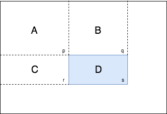
</p>

<p><img src="https://chamoda.com/assets/posts/realtime-face-detection-using-opencv-and-python/sum.png" alt="Integral sum" /></p>

<p>We know values p, q, r, s in the integral image and they represent the sum of all the left and top values. Our goal is to find the pixel sum of D.</p>

\[p = A \\
q = A + B \\
r = A + C \\
s = A + B + C + D \\\]

<p>So \(D = (p + s) - (q + r)\) which will reduce computation steps to calculate the sum of pixels in the defined rectangle significantly.</p>

<p>Here’s the equivalent python code.</p>

<div class="language-python highlighter-rouge"><div class="highlight"><pre class="highlight"><code><span class="k">def</span> <span class="nf">sum_region</span><span class="p">(</span><span class="n">integral_img</span><span class="p">,</span> <span class="n">top_left</span><span class="p">,</span> <span class="n">bottom_right</span><span class="p">):</span>
    <span class="c1"># to numpy matrix notation
</span>    <span class="n">top_left</span> <span class="o">=</span> <span class="p">(</span><span class="n">top_left</span><span class="p">[</span><span class="mi">1</span><span class="p">],</span> <span class="n">top_left</span><span class="p">[</span><span class="mi">0</span><span class="p">])</span> 
    <span class="n">bottom_right</span> <span class="o">=</span> <span class="p">(</span><span class="n">bottom_right</span><span class="p">[</span><span class="mi">1</span><span class="p">],</span> <span class="n">bottom_right</span><span class="p">[</span><span class="mi">0</span><span class="p">])</span>
    <span class="k">if</span> <span class="n">top_left</span> <span class="o">==</span> <span class="n">bottom_right</span><span class="p">:</span>
        <span class="k">return</span> <span class="n">integral_img</span><span class="p">[</span><span class="n">top_left</span><span class="p">]</span>
    <span class="n">top_right</span> <span class="o">=</span> <span class="p">(</span><span class="n">bottom_right</span><span class="p">[</span><span class="mi">0</span><span class="p">],</span> <span class="n">top_left</span><span class="p">[</span><span class="mi">1</span><span class="p">])</span>
    <span class="n">bottom_left</span> <span class="o">=</span> <span class="p">(</span><span class="n">top_left</span><span class="p">[</span><span class="mi">0</span><span class="p">],</span> <span class="n">bottom_right</span><span class="p">[</span><span class="mi">1</span><span class="p">])</span>
    <span class="c1"># s + p - (q + r)
</span>    <span class="k">return</span> <span class="n">integral_img</span><span class="p">[</span><span class="n">bottom_right</span><span class="p">]</span> <span class="o">+</span> <span class="n">integral_img</span><span class="p">[</span><span class="n">top_left</span><span class="p">]</span> <span class="o">-</span> <span class="n">integral_img</span><span class="p">[</span><span class="n">top_right</span><span class="p">]</span> <span class="o">-</span> <span class="n">integral_img</span><span class="p">[</span><span class="n">bottom_left</span><span class="p">]</span>    
</code></pre></div></div>

<h2 id="adaboost-adaptive-boosting">AdaBoost (Adaptive Boosting)</h2>

<p>Now we need a way to select best features from all possible features that can correctly classify a face. AdaBoost algorithm was formulated by Yoav Freund and Robert Schapire in 1997 and won the prestigious <a href="https://en.wikipedia.org/wiki/G%C3%B6del_Prize">Gödel Prize</a> in 2003. This elegant machine learning approach can be applied to wide range of problems not only image detection.</p>

<p>I’ll start with the idea of weak and strong classifiers.</p>

<ul>
  <li>Weak Classifier - Classifier that’s little bit better than random guessing.</li>
  <li>Strong Classifier - A combination of weak classifiers. It represents wisdom of a weighted crowd of experts.</li>
</ul>

<p>AdaBoost itself is an inherently incomplete algorithm, so it’s called a meta algorithm. Let’s express the idea of strong classifier mathematically.</p>

\[H(x) = sign\Big( h_1(x) + h_2(x) +  ... +h_T(x)\Big)\]

<p>H(x) is a strong classifier which classify according to the sign of the sum of weak classifiers. Every weak classifier is a Haar feature combined with some other parameters I’ll detail in the next few paragraphs. Suppose there are only 3 weak classifiers so \(T = 3\). Every classifier outputs +1 or -1 so sum of weak classifier will have either + or - sign.</p>

\[H(x) = sign\Big( +1 + -1 + -1 \Big)\]

<p>Here the strong classifier sign is negative so it may not be a face. I started with this analogy but we have to also weight the weak classifiers because some classifiers may have stronger influence than others.</p>

<p>By adding weights the strong classifier gets a little complicated but it’s nothing more than a simple inequality match.</p>

\[H(x) = \begin{cases}
      +1, \text{if}\ \sum_{t = 1}^{T} \alpha_th_t(x) \ge \frac{1}{2} \sum_{t = 1}^{T} \alpha_t \\
      -1, \text{otherwise}
     \end{cases}\]

<p>Now how do we decide which weak classifier to use, which \(\alpha\) weights to use? That’s why we need to train over existing labeled data. Suppose image is \(x_i\) and label is \(y_i\) which is 1 for face and 0 for non face. Given example images \((x_1, y_1), ... , (x_m, y_m)\) we will initialize weights for each example. Don’t confuse this weight with the \(\alpha\) weight discussed before. This algorithm has two kind of weights. One is \(\alpha\) weight for selected weak classifier. Other one is for each example and each step denoted by \(w_{t,i}\). Now we are going to intialize weights mentioned later for step one \(t = 1\)</p>

\[w_{1, i} = \frac{1}{m}\]

<p>Here we have normalized the weights so the sum of the weights is 1. We do the normalization in every step to make sure the weight distribution always adds up to 1.</p>

\[\sum_{i = 1}^{m} w_{t, i} = 1\]

<p>The generalized normalized equation is</p>

\[w_{t,i} = \frac{w_{t,i}}{\sum_{j = 0}^{m}w_{t,i}}\]

<p>Next we loop over all the features to select the best weak classifier which minimize error rate.</p>

\[\epsilon_t = min_{f, p, \theta} \sum_{i = 1}^m w_{t, i} | h(x_i, f, p, \theta) - y_i |\]

<p>Here we are calculating the sum of weights of misclassified examples which is the error rate represented by epsilon \(\epsilon\). Notice \(h(x_i, f, p, \theta) - y_i\) returns 1 or -1 if misclassified, 0 if correctly classified. We are taking the absolute value out of it so the weight gets multiplied by 1 if misclassified. Let’s dive into the definition of weak classifier.</p>

\[h(x) = h(x_i, f, p, \theta)\]

<p>\(x_i\) is the \(i\)‘th image example. \(f\) is the Haar feature. \(p\) is the polarity which is either -1 or +1 which defines direction of the inequality. \(\theta\) is the threshold.</p>

\[h(x, f, p , \theta) = \begin{cases}
	1, \text{if } pf(x) \lt p\theta \\
      	0, \text{otherwise}
     	\end{cases}\]

<p>To select the \(f\) feature we need to loop over f(x) Haar classifier. To select the threshold we need to minimize the following equation.</p>

\[error_{\theta} = min\Big( (S_+) + (T_-) - (S_-), (S_-) + (T_+) - (S_+))\Big)\]

<p>Here’s the definition of symbols</p>

<ul>
  <li>\(T_+\) is total sum of positive sample weights</li>
  <li>\(T_-\) is total sum of negative sample weights</li>
  <li>\(S_+\) is sum of positive sample weights below threshold</li>
  <li>\(S_-\) is sum of negative sample weights below threshold</li>
</ul>

<p>After finding the minimized error \(\epsilon_t\) for step \(t\) we can find the weights for the next step \(t + 1\)</p>

\[w_{t+1, i} = w_{t, i} \Big(\frac{\epsilon_t}{1 - \epsilon_t}\Big)^{1 -e_i}\]

<p>Where \(e_i = 0\) if sample image \(x_i\) is correctly classified, 1 otherwise. The goal of the equation is to make the weights of incorrectly classified samples slightly larger so in the next round it will be unforgiving to weak classifiers that are going to classify the same samples incorrectly. So in each step it’s going to choose a unique weak classifier with a unique feature. To do so in the above equation correctly classified weights will be decreased so misclassified weights will increase relative to correct weights.</p>

<p>Finally calculate \(\alpha_t\) for the selected classifier.</p>

\[\alpha_t = log(\frac{1 - \epsilon_t}{\epsilon_t})\]

<p>Notice how \(\alpha\) is going to be a higher value if the error rate is small so that weak classifier has more contribution to the strong classifier.</p>

<p>So finally the algorithm needs to loop \(T\) steps to find \(T\) classifiers to get good results.</p>

<h2 id="cascading">Cascading</h2>

<p>
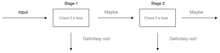
You may have noticed how many loops we have in the algorithm so this AdaBoost along with Haar Features is computationally expensive for real time detection. So we are using an attentional cascade to reduce some unnecessary computations. A more efficient cascade can be constructed so that negative sub-windows will be rejected early. Every stage of the cascade is a strong classifier, so all the features are grouped into several stages where each stage has several features.</p>

<p><img src="https://chamoda.com/assets/posts/realtime-face-detection-using-opencv-and-python/cascade.png" alt="Cascade" /></p>

<p>For the cascade we need the following parameters</p>

<ul>
  <li>Number of stages in cascade</li>
  <li>Number of features in each cascade</li>
  <li>Threshold of each strong classifier</li>
</ul>

<p>Finding optimum values for above parameters is a difficult task. Viola Jones introduced a simple method to find the optimum combination.</p>

<ul>
  <li>Select \(f_i\) the maximum acceptable false positive rate per stage</li>
  <li>Select \(d_i\) the maximum acceptable true positive rate per stage</li>
  <li>Select \(F_{target}\) Overall false positive rate</li>
</ul>

<p>Now we are looping until the predefined \(F_{target}\) is met by adding new stages. In stages we keep adding features until \(f_i\) and \(d_i\) are met. By doing this we are going to create a cascade of strong classifiers.</p>

<h2 id="additional-resources">Additional resources</h2>

<ul>
  <li>Paper (Revised) <a href="http://www.vision.caltech.edu/html-files/EE148-2005-Spring/pprs/viola04ijcv.pdf">Viola Jones 2001</a>.</li>
  <li>Viola Jones Python Implementation <a href="https://github.com/Simon-Hohberg/Viola-Jones">GitHub</a></li>
  <li>To learn more about AdaBoost read the  book <a href="https://www.amazon.com/Boosting-Foundations-Algorithms-Adaptive-Computation/dp/0262526034">Boosting Foundations and Algorithms</a>. It’s written by the original authors of the algorithm.</li>
  <li>Source code for the face detection in this post - <a href="https://github.com/chamoda/realtime-face-detection">Realtime face detection</a></li>
  <li>Pull requests are welcome if you find anything wrong in the post - <a href="https://github.com/chamoda/chamoda.github.io">Blog</a></li>
</ul>]]></content><author><name></name></author><summary type="html"><![CDATA[Learn how to implement real-time face detection using OpenCV and Python with the Viola-Jones algorithm. Complete tutorial with code examples and Haar cascades.]]></summary></entry><entry><title type="html">Introduction to machine learning with linear regression</title><link href="https://chamoda.com/introduction-to-machine-learning-with-linear-regression" rel="alternate" type="text/html" title="Introduction to machine learning with linear regression" /><published>2017-10-05T00:00:00+00:00</published><updated>2017-10-05T00:00:00+00:00</updated><id>https://chamoda.com/introduction-to-machine-learning-with-linear-regression</id><content type="html" xml:base="https://chamoda.com/introduction-to-machine-learning-with-linear-regression"><![CDATA[<p>Machine learning is all about computers learning from data to predict new data. There are two types of categories in machine learning</p>

<ul>
  <li>Supervised Learning</li>
  <li>Unsupervised Learning</li>
</ul>

<p>In supervised learning computer learns from input and output while creating a general model which can be used to predict output from new input. Unsupervised learning is about discovering patterns in data without knowing explicit labels beforehand. In this post I’m going to talk about linear regression which is a supervised learning method.</p>

<h2 id="jupyter-notebook">Jupyter Notebook</h2>

<p>Jupyter Notebook is an interactive python environment. You can install jupyter notebook with <a href="https://www.anaconda.com/download">Anaconda</a> which will also install all necessary packages. After installation just run <code class="language-plaintext highlighter-rouge">jupyter notebook</code> in command line, which will open jupyter notebook instance in browser. Click <code class="language-plaintext highlighter-rouge">New</code> and create a Python 2 notebook.</p>

<p>Enter following lines of code in the cell and press <code class="language-plaintext highlighter-rouge">Shift + Enter</code> which will execute the code. Full notebook of the code I used in this post is also available on <a href="https://github.com/chamoda/LinearRegression">github</a>.</p>

<div class="language-python highlighter-rouge"><div class="highlight"><pre class="highlight"><code><span class="kn">import</span> <span class="nn">numpy</span> <span class="k">as</span> <span class="n">np</span>
<span class="kn">import</span> <span class="nn">matplotlib.pyplot</span> <span class="k">as</span> <span class="n">plt</span>
</code></pre></div></div>

<p><a href="http://www.numpy.org/">Numpy</a> is used for matrix operations. It’s the most important library in python scientific computing ecosystem.</p>

<p><a href="https://matplotlib.org/">Matplotlib</a> is a plotting library. We will use it to visualize our data.</p>

<h2 id="data">Data</h2>

<p>In this post I’m not going to use any real data set. Instead I’m going to generate some random data.</p>

<div class="language-python highlighter-rouge"><div class="highlight"><pre class="highlight"><code><span class="n">rng</span> <span class="o">=</span> <span class="n">np</span><span class="p">.</span><span class="n">random</span><span class="p">.</span><span class="n">RandomState</span><span class="p">(</span><span class="mi">42</span><span class="p">)</span>
<span class="n">x</span> <span class="o">=</span> <span class="n">rng</span><span class="p">.</span><span class="n">rand</span><span class="p">(</span><span class="mi">100</span><span class="p">)</span> <span class="o">*</span> <span class="mi">10</span>
<span class="n">x</span> <span class="o">=</span> <span class="n">x</span><span class="p">[:,</span> <span class="n">np</span><span class="p">.</span><span class="n">newaxis</span><span class="p">]</span>
<span class="n">b</span> <span class="o">=</span> <span class="n">rng</span><span class="p">.</span><span class="n">rand</span><span class="p">(</span><span class="mi">100</span><span class="p">)</span> <span class="o">*</span> <span class="mi">5</span>
<span class="n">b</span> <span class="o">=</span> <span class="n">b</span><span class="p">[:,</span> <span class="n">np</span><span class="p">.</span><span class="n">newaxis</span><span class="p">]</span>
<span class="n">y</span> <span class="o">=</span> <span class="mi">3</span> <span class="o">*</span> <span class="n">x</span> <span class="o">+</span> <span class="n">b</span>
</code></pre></div></div>

<p>Here we generate 100 rows of random data we will say \(m = 100\). \(m\) is usually used in machine learning to denote number of data, in this case pairs of \(x\) and \(y\). Now we are going to plot the dataset using Matplotlib.</p>

<div class="language-python highlighter-rouge"><div class="highlight"><pre class="highlight"><code><span class="n">plt</span><span class="p">.</span><span class="n">scatter</span><span class="p">(</span><span class="n">x</span><span class="p">,</span> <span class="n">y</span><span class="p">)</span>
<span class="n">plt</span><span class="p">.</span><span class="n">xlabel</span><span class="p">(</span><span class="s">'x axis'</span><span class="p">)</span>
<span class="n">plt</span><span class="p">.</span><span class="n">ylabel</span><span class="p">(</span><span class="s">'y axis'</span><span class="p">)</span>
<span class="n">plt</span><span class="p">.</span><span class="n">show</span><span class="p">()</span>
</code></pre></div></div>

<p>This is the plot generated from the code. Every blue dot is a data point. There are 100 blue dots here.</p>

<p><img src="https://chamoda.com/assets/posts/linear-regression/plot.png" alt="plot" /></p>

<p>Data is distributed in a sort of linear nature because of the way we generate random data.</p>

<h2 id="linear-regression">Linear regression</h2>

<p>So the purpose of linear regression is to find the equation of a line that does justice to all data points. We will define the equation of the line as \(h(x) = \theta_0 + \theta_1x\). In machine learning \(h(x)\) is called the hypothesis function. But this is just a fancy way of writing old school \(y = mx + c\) where \(c = \theta_0\) and \(m = \theta_1\). Now our goal is to find \(\theta_0\) and \(\theta_1\). If we know the \(\theta_0\) and \(\theta_1\) we can draw the line. To find \(\theta_0\) and \(\theta_1\) we are going to use a function called cost function.</p>

<h2 id="cost-function">Cost function</h2>

<p>We are going to use the following equation which is called the least square method.</p>

\[J(\theta_0, \theta_1) = \frac{1}{2m}\sum_{i=1}^m(h(x^{(i)}) - y^{(i)})^2\]

<p>The goal is to minimize \((h(x) - y)\) so the difference between the hypothesis function output and \(y\) is minimized as much as possible. Suppose \(\sum_{i=1}^m(h(x^{(i)}) - y^{(i)})^2\) is \(0\), that means \(J(\theta_0, \theta_1) = 0\) so data will fit perfectly to the straight line \(h(x) = \theta_0 + \theta_1x\). But for a real dataset that may not be the case. If data has spread all over the plot this value may be high. Ok, you get now what \((h(x) - y)\) means but why squaring it? We square it because there could be negative or positive values for \(h(x^{(i)}) - y^{(i)}\) depending on the way data is distributed when using a range of values for \(\theta_0\) and \(\theta_1\). By squaring we make sure there are no negative values so there is no cancelling out situations. By that means \(0\) really means that it fits the data distribution. In a real world situation if data is not perfectly linear we can’t get \(J(\theta_0, \theta_1)\) to zero but try to get a minimum value possible. We say this as ‘minimizing the cost function’. We divide by \(m\) to get a relatively small value. We divided by 2 because, by a future derivative operation another function will be a much simpler equation.</p>

<p>Now we are going to implement the cost function in python. First we implement the hypothesis function \(h(x) = \theta_0 + \theta_1x\).</p>

<div class="language-python highlighter-rouge"><div class="highlight"><pre class="highlight"><code><span class="k">def</span> <span class="nf">h</span><span class="p">(</span><span class="n">x</span><span class="p">,</span> <span class="n">theta0</span><span class="p">,</span> <span class="n">theta1</span><span class="p">):</span>
    <span class="k">return</span> <span class="n">theta0</span> <span class="o">+</span> <span class="n">theta1</span> <span class="o">*</span> <span class="n">x</span>
</code></pre></div></div>

<p>If we pass normal python integer values to <code class="language-plaintext highlighter-rouge">x</code>, <code class="language-plaintext highlighter-rouge">theta0</code>, <code class="language-plaintext highlighter-rouge">theta1</code> it will output an integer. What will happen if we change <code class="language-plaintext highlighter-rouge">x</code> to a numpy array? All values get multiplied by <code class="language-plaintext highlighter-rouge">theta1</code>, then all values will get added by <code class="language-plaintext highlighter-rouge">theta0</code>. Output will be a numpy array. This happens because of a python feature called broadcasting. It will save us from writing a for loop to calculate all the values step by step. Broadcasting is a very powerful concept. Use of broadcasting will be used everywhere when doing machine learning in python. Next we implement the cost function in python</p>

<div class="language-python highlighter-rouge"><div class="highlight"><pre class="highlight"><code><span class="k">def</span> <span class="nf">cost</span><span class="p">(</span><span class="n">x</span><span class="p">,</span> <span class="n">theta0</span><span class="p">,</span> <span class="n">theta1</span><span class="p">):</span>
    <span class="k">return</span> <span class="n">np</span><span class="p">.</span><span class="nb">sum</span><span class="p">(</span><span class="n">np</span><span class="p">.</span><span class="n">power</span><span class="p">(</span><span class="n">h</span><span class="p">(</span><span class="n">x</span><span class="p">,</span> <span class="n">theta0</span><span class="p">,</span> <span class="n">theta1</span><span class="p">)</span> <span class="o">-</span> <span class="n">y</span><span class="p">,</span> <span class="mi">2</span><span class="p">))</span> <span class="o">*</span> <span class="mi">1</span> <span class="o">/</span> <span class="mi">2</span> <span class="o">*</span> <span class="n">x</span><span class="p">.</span><span class="n">shape</span><span class="p">[</span><span class="mi">0</span><span class="p">]</span>
</code></pre></div></div>

<p><code class="language-plaintext highlighter-rouge">np.sum()</code> function takes the sum of all the values inside a numpy array and returns a scalar value. <code class="language-plaintext highlighter-rouge">np.power()</code> takes power, in this case square of all the values and returns a same size array with modified values. We pass a numpy array as <code class="language-plaintext highlighter-rouge">x</code> so <code class="language-plaintext highlighter-rouge">x.shape[0]</code> is the number of elements in <code class="language-plaintext highlighter-rouge">x</code> which is also equal to \(m\).</p>

<p>Now we need to find <code class="language-plaintext highlighter-rouge">theta0</code> and <code class="language-plaintext highlighter-rouge">theta1</code> which minimize the cost function. One approach is to brute force a range of <code class="language-plaintext highlighter-rouge">theta0</code> and <code class="language-plaintext highlighter-rouge">theta1</code> and pick values where the return value of the cost function is minimal. But can we do better?</p>

<h2 id="gradient-descent">Gradient descent</h2>

<p>Gradient descent is an iterative algorithm to find out the minimum of a function. This is what we are going to do.</p>

\[\theta_0 := \theta_0 - \alpha \frac{\partial}{\partial \theta_0} J(\theta_0, \theta_1)\]

\[\theta_1 := \theta_1 - \alpha \frac{\partial}{\partial \theta_1} J(\theta_0, \theta_1)\]

<p>I will explain step by step. First \(:=\) is the assignment operator. In programming languages we use \(=\) operator but in math it means equality. So \(:=\) means assignment in mathematics. \(\alpha\) is called the learning rate which I will explain later in detail. \(\frac{\partial}{\partial \theta_0} J(\theta_0, \theta_1)\) is called the derivative part.</p>

\[\frac{\partial}{\partial \theta_0} J(\theta_0, \theta_1) = \frac{\partial}{\partial \theta_0} \frac{1}{2m}\sum_{i=1}^m(h(x^{(i)}) - y^{(i)})^2\]

<p>This is what the plot looks with \(\theta_0\) against cost function like after 100,000 iterations.</p>

<p><img src="https://chamoda.com/assets/posts/linear-regression/theta0_cost.png" alt="plot" /></p>

<p>Derivative is measuring the slope, You can see the slope is a negative value as the plot going down. \(\alpha\) is the learning rate which is \(0.0001\). So</p>

\[\theta_0 := \theta_0 - \alpha \frac{\partial}{\partial \theta_0} J(\theta_0, \theta_1)\]

<p>You can see \(\theta_0\) will increase because \(\alpha\) is positive and \(\frac{\partial}{\partial \theta_0} J(\theta_0, \theta_1)\) is negative. Rate of change in slope is decreasing so \(\theta_0\) will become a stabilized value.</p>

<p>Here’s the derivative steps for \(\theta_0\).</p>

\[\frac{\partial}{\partial \theta_0} J(\theta_0, \theta_1)  = \frac{1}{2m} \frac{\partial}{\partial \theta_0} \sum_{i=1}^m(h(x^{(i)}) - y^{(i)})^2\]

<p>I’ve taken out the \(\frac{1}{2m}\) out of the derivative. Since \(h(x^{(i)}) = \theta_0 + \theta_1x^{(i)}\) we can write</p>

\[\frac{\partial}{\partial \theta_0} J(\theta_0, \theta_1)  = \frac{1}{2m} \frac{\partial}{\partial \theta_0} \sum_{i=1}^m(\theta_0 + \theta_1x^{(i)} - y^{(i)})^2\]

<p>Now we are ready to take the derivative.</p>

\[\frac{\partial}{\partial \theta_0} J(\theta_0, \theta_1)  = \frac{1}{m} \sum_{i=1}^m(\theta_0 + \theta_1x^{(i)} - y^{(i)})\]

<p>Next derivative steps for \(\theta_1\).</p>

\[\frac{\partial}{\partial \theta_1} J(\theta_0, \theta_1)  = \frac{1}{2m} \frac{\partial}{\partial \theta_1} \sum_{i=1}^m(h(x^{(i)}) - y^{(i)})^2\]

\[\frac{\partial}{\partial \theta_1} J(\theta_0, \theta_1)  = \frac{1}{2m} \frac{\partial}{\partial \theta_1} \sum_{i=1}^m(\theta_0 + \theta_1x^{(i)} - y^{(i)})^2\]

<p>After taking the derivative,</p>

\[\frac{\partial}{\partial \theta_1} J(\theta_0, \theta_1)  = \frac{1}{m} \sum_{i=1}^m(\theta_0 + \theta_1x^{(i)} - y^{(i)})x^{(i)}\]

<p>Now let’s look at the equivalent python code.</p>

<div class="language-python highlighter-rouge"><div class="highlight"><pre class="highlight"><code><span class="n">theta0</span> <span class="o">=</span> <span class="mi">0</span>
<span class="n">theta1</span> <span class="o">=</span> <span class="mi">0</span>
<span class="n">alpha</span> <span class="o">=</span> <span class="mf">0.001</span>
<span class="n">iteration</span> <span class="o">=</span> <span class="mi">0</span>

<span class="k">while</span> <span class="bp">True</span><span class="p">:</span>    
    <span class="n">temp0</span> <span class="o">=</span> <span class="p">(</span><span class="mi">1</span> <span class="o">/</span> <span class="n">m</span><span class="p">)</span> <span class="o">*</span> <span class="n">np</span><span class="p">.</span><span class="nb">sum</span><span class="p">(</span><span class="n">h</span><span class="p">(</span><span class="n">x</span><span class="p">,</span> <span class="n">theta0</span><span class="p">,</span> <span class="n">theta1</span><span class="p">)</span> <span class="o">-</span> <span class="n">y</span><span class="p">)</span>
    <span class="n">temp1</span> <span class="o">=</span> <span class="p">(</span><span class="mi">1</span> <span class="o">/</span> <span class="n">m</span><span class="p">)</span> <span class="o">*</span> <span class="n">np</span><span class="p">.</span><span class="nb">sum</span><span class="p">((</span><span class="n">h</span><span class="p">(</span><span class="n">x</span><span class="p">,</span> <span class="n">theta0</span><span class="p">,</span> <span class="n">theta1</span><span class="p">)</span> <span class="o">-</span> <span class="n">y</span><span class="p">)</span> <span class="o">*</span> <span class="n">x</span><span class="p">)</span>
    
    <span class="n">theta0</span> <span class="o">=</span> <span class="n">theta0</span> <span class="o">-</span> <span class="n">alpha</span> <span class="o">*</span> <span class="n">temp0</span>
    <span class="n">theta1</span> <span class="o">=</span> <span class="n">theta1</span> <span class="o">-</span> <span class="n">alpha</span> <span class="o">*</span> <span class="n">temp1</span>
        
    <span class="n">iteration</span> <span class="o">+=</span> <span class="mi">1</span>
    
    <span class="k">if</span> <span class="n">iteration</span> <span class="o">&gt;</span> <span class="mi">100000</span><span class="p">:</span>
        <span class="k">print</span><span class="p">(</span><span class="s">"theta0: "</span> <span class="o">+</span> <span class="nb">str</span><span class="p">(</span><span class="n">theta0</span><span class="p">)</span> <span class="o">+</span> <span class="s">"theta1:"</span> <span class="o">+</span> <span class="nb">str</span><span class="p">(</span><span class="n">theta1</span><span class="p">))</span>
        <span class="k">break</span>
</code></pre></div></div>

<p>We are initializing <code class="language-plaintext highlighter-rouge">theta0</code> and <code class="language-plaintext highlighter-rouge">theta1</code> to 0. Learning rate <code class="language-plaintext highlighter-rouge">alpha</code> to be <code class="language-plaintext highlighter-rouge">0.001</code>. You must choose a smaller value or else it may not converge smoothly. Also note that you must use temporary values while assigning.</p>

<p>Now that we have found optimal <code class="language-plaintext highlighter-rouge">theta0</code> and <code class="language-plaintext highlighter-rouge">theta1</code> values below, we draw a line on top of the first plot.</p>

<div class="language-plaintext highlighter-rouge"><div class="highlight"><pre class="highlight"><code>theta0: 2.567988282theta1:2.98323417806
</code></pre></div></div>

<p><img src="https://chamoda.com/assets/posts/linear-regression/final.png" alt="plot" /></p>

<p>You can see that the algorithm learned to draw the most optimal line over the data distribution.</p>

<h2 id="prediction">Prediction</h2>

<p>Here comes the easy part. Now we have a model with learned parameters which can be used to predict. We can use our hypothesis function.</p>

<div class="language-python highlighter-rouge"><div class="highlight"><pre class="highlight"><code><span class="n">y</span> <span class="o">=</span> <span class="n">h</span><span class="p">(</span><span class="mi">3</span><span class="p">,</span> <span class="n">theta1</span><span class="p">,</span> <span class="n">theta2</span><span class="p">)</span>
</code></pre></div></div>

<div class="language-plaintext highlighter-rouge"><div class="highlight"><pre class="highlight"><code>11.517690816184686
</code></pre></div></div>

<h2 id="scikit-learn">Scikit-learn</h2>

<p>Scikit Learn is a python library with one of the most used classical machine learning algorithms. Now you know what happens under the hood of the linear regression function. So you are ready to use a library to do production level linear regression machine learning.</p>

<p>Here’s how you import the library</p>

<div class="language-python highlighter-rouge"><div class="highlight"><pre class="highlight"><code><span class="kn">from</span> <span class="nn">sklearn.linear_model</span> <span class="kn">import</span> <span class="n">LinearRegression</span>
</code></pre></div></div>

<div class="language-python highlighter-rouge"><div class="highlight"><pre class="highlight"><code><span class="n">model</span> <span class="o">=</span> <span class="n">LinearRegression</span><span class="p">()</span>
<span class="n">model</span><span class="p">.</span><span class="n">fit</span><span class="p">(</span><span class="n">x</span><span class="p">,</span> <span class="n">y</span><span class="p">)</span>
</code></pre></div></div>

<p><code class="language-plaintext highlighter-rouge">fit()</code> function trains the data.</p>

<div class="language-python highlighter-rouge"><div class="highlight"><pre class="highlight"><code><span class="n">model</span><span class="p">.</span><span class="n">predict</span><span class="p">(</span><span class="mi">3</span><span class="p">)</span>
</code></pre></div></div>

<div class="language-plaintext highlighter-rouge"><div class="highlight"><pre class="highlight"><code>11.51769082
</code></pre></div></div>

<p>You can see that the values are similar to our own implementation.</p>

<p>GitHub repo of example code is available <a href="https://github.com/chamoda/linear-regression">here</a></p>]]></content><author><name></name></author><summary type="html"><![CDATA[Learn the basics of machine learning with linear regression - covering supervised vs unsupervised learning, data visualization with Python, and implementing gradient descent from scratch.]]></summary></entry></feed>