Introduction to Machine Learning with Linear Regression
Machine learning is all about computers learning itself from data to predict new data. There are two types of categories in machine learning
- Supervised Learning
- Unsupervised Learning
In supervised learning computer learns from input and output while creating a general model which can be used to predict output from new input. Unsupervised learning is about discovering pattern in data without knowing explicit labels beforehand. In this post I’m going to talk about linear regression which is a supervised learning method.
Jupyter Notebook
Jupyter Notebook is an interactive python environment. You can install jupyter notebook with Anaconda which will also install all necessary packages. After installation just run jupyter notebook in command line, which will open jupyter notebook instance in browser. Click New and create a Python 2 notebook.
Enter following lines of code in the cell and press Shift + Enter which will execute the code. Full notebook of the code I used in this post is also available on github.
import numpy as np
import matplotlib.pyplot as plt
Numpy is used for matrix operations. It’s the most important library in python scientific computing echo system.
Matplotlib is a plotting library. We will use it to visualize our data.
Data
In this post I’m not going to use any real data set. Instead I’m going to generate some random data.
rng = np.random.RandomState(42)
x = rng.rand(100) * 10
x = x[:, np.newaxis]
b = rng.rand(100) * 5
b = b[:, np.newaxis]
y = 3 * x + b
Here we generate 100 rows of random data we will say \(m = 100\). \(m\) is usually used in machine learning to denote number of data, in this case pairs of \(x\) and \(y\). Now we are going to plot the dataset using Matplotlib.
plt.scatter(x, y)
plt.xlabel('x axis')
plt.ylabel('y axis')
plt.show()
This is the plot generate from the code. Every blue dot is a data point. There are 100 blue dots here.
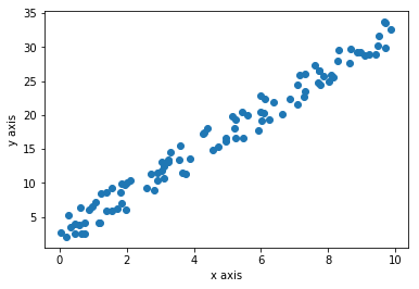
Data is distributed in sort of linear nature because of the way we generate random data.
Linear Regression
So purpose of the linear regression is to find the equation of a line that do justice to all data points. We will define the equation of the line as \(h(x) = \theta_0 + \theta_1x\). In machine learning \(h(x)\) is called the hypothesis function. But this is just a fancy way of writing old school \(y = mx + c\) where \(c = \theta_0\) and \(m = \theta_1\). Now our goal is to find find \(\theta_0\) and \(\theta_1\). If we know the \(\theta_0\) and \(\theta_1\) we can draw the line. To find \(\theta_0\) and \(\theta_1\) we are going to use a function called cost function.
Cost Function
We going to use following equation which is called least square method.
\[J(\theta_0, \theta_1) = \frac{1}{2m}\sum_{i=1}^m(h(x^{(i)}) - y^{(i)})^2\]Goal is to minimize \((h(x) - y)\) so difference between the hypothesis function output and \(y\) is minimized as possible. Suppose \(\sum_{i=1}^m(h(x^{(i)}) - y^{(i)})^2\) is \(0\), that means \(J(\theta_0, \theta_1) = 0\) so data will fit perfectly to the strait line \(h(x) = \theta_0 + \theta_1x\). But for a real dataset that may be not the case. If data has spread all over the plot this value may be hight. Ok, you get now what \((h(x) - y)\) means but why squaring it? We sqaure it because there could be negetive or positive values for \(h(x^{(i)}) - y^{(i)}\) depending on the the way data is distributetd when using range of values for \(\theta_0\) and \(\theta_1\). By squaring we make sure there is no negetive values so their is no cancelling out situations. By that means \(0\) realy means that it’s fit the data distrubbution. In a real world situation if data is not perfectly linear we can’t get \(J(\theta_0, \theta_1)\) to zero but try to get a minimum value possible. We say this as ‘minimizing the cost function’. We divide by \(m\) get a relatively small value. We devided by 2 because, by a future derivative operation anther function will a be much simpler equation.
Now we are going to implement the cost function in python. First we implement the hypothesis function \(h(x) = \theta_0 + \theta_1x\).
def h(x, theta0, theta1):
    return theta0 + theta1 * x
If we pass normal python integer values to x, theta0, theta1 it will output an integer. What will happen if we change x to a numpy array. All values get multiplied by theta1, then all values will get added by theta0. Output will be a numpy array. This happens because of a python feature called broadcasting. It will save us from writing a for loop to calculate all the values step by step. Broadcastng is a very powerpull concept. Use of broadcasting will be used everywhere when doing machine learning in python. Next we implement cost function in python
def cost(x, theta0, theta1):
    return np.sum(np.power(h(x, theta0, theta1) - y, 2)) * 1 / 2 * x.shape[0]
np.sum() function take sum of all the values inside a numpy array and return a scaler value. np.power() take power, in this case square of all the values and retrun a same size array with modified values. we pass a numpy array as x so x.shape[0] is number of elements in x which is also equal to \(m\).
Now we need to find theta0 and theta1 which minimize the cost function. One approach is to brute force a range of theta0 and theta1 and pick values where return value of cost function is minimal. But can we to better?
Gradient Descent
Gradient descent is an iterative algorithm to find out the minimum of a function. This is what we are going to do.
\[\theta_0 := \theta_0 - \alpha \frac{\partial}{\partial \theta_0} J(\theta_0, \theta_1)\] \[\theta_1 := \theta_1 - \alpha \frac{\partial}{\partial \theta_1} J(\theta_0, \theta_1)\]I will explain step by step. First \(:=\) is the assignment operator. In programming languages we use \(=\) operator but in math it means equality. So \(:=\) means assignment in mathematics. \(\alpha\) is called the learning rate which I will explain later in detail. \(\frac{\partial}{\partial \theta_0} J(\theta_0, \theta_1)\) is called the derivative part.
\[\frac{\partial}{\partial \theta_0} J(\theta_0, \theta_1) = \frac{\partial}{\partial \theta_0} \frac{1}{2m}\sum_{i=1}^m(h(x^{(i)}) - y^{(i)})^2\]This is what the plot looks with \(\theta_0\) against cost function like after 100,000 iterations.
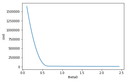
Derivative is measuring the slope, You can see the slope is a negative value as the plot going down. \(\alpha\) is the learning rate which is \(0.0001\). So
\[\theta_0 := \theta_0 - \alpha \frac{\partial}{\partial \theta_0} J(\theta_0, \theta_1)\]You can see \(\theta_0\) will increase because \(\alpha\) is positive \(\frac{\partial}{\partial \theta_0} J(\theta_0, \theta_1)\) is negative. Rate of change in lope is decreasing so \(\theta_0\) will become a stabilized value.
Here’s the derivative steps for \(\theta_0\).
\[\frac{\partial}{\partial \theta_0} J(\theta_0, \theta_1) = \frac{1}{2m} \frac{\partial}{\partial \theta_0} \sum_{i=1}^m(h(x^{(i)}) - y^{(i)})^2\]I’ve taken out the \(\frac{1}{2m}\) out of the derivative. Since \(h(x^{(i)}) = \theta_0 + \theta_1x^{(i)}\) we can write
\[\frac{\partial}{\partial \theta_0} J(\theta_0, \theta_1) = \frac{1}{2m} \frac{\partial}{\partial \theta_0} \sum_{i=1}^m(\theta_0 + \theta_1x^{(i)} - y^{(i)})^2\]Now we are ready to take the derivative.
\[\frac{\partial}{\partial \theta_0} J(\theta_0, \theta_1) = \frac{1}{m} \sum_{i=1}^m(\theta_0 + \theta_1x^{(i)} - y^{(i)})\]Next derivative steps for \(\theta_1\).
\[\frac{\partial}{\partial \theta_1} J(\theta_0, \theta_1) = \frac{1}{2m} \frac{\partial}{\partial \theta_1} \sum_{i=1}^m(h(x^{(i)}) - y^{(i)})^2\] \[\frac{\partial}{\partial \theta_1} J(\theta_0, \theta_1) = \frac{1}{2m} \frac{\partial}{\partial \theta_1} \sum_{i=1}^m(\theta_0 + \theta_1x^{(i)} - y^{(i)})^2\]After taking the derivative,
\[\frac{\partial}{\partial \theta_1} J(\theta_0, \theta_1) = \frac{1}{m} \sum_{i=1}^m(\theta_0 + \theta_1x^{(i)} - y^{(i)})x^{(i)}\]Now let’s look at the equivalent python code.
theta0 = 0
theta1 = 0
alpha = 0.001
iteration = 0

while True:
    temp0 = (1 / m) * np.sum(h(x, theta0, theta1) - y)
    temp1 = (1 / m) * np.sum((h(x, theta0, theta1) - y) * x)

    theta0 = theta0 - alpha * temp0
    theta1 = theta1 - alpha * temp1

    iteration += 1

    if iteration > 100000:
        print("theta0: " + str(theta0) + "theta1:" + str(theta1))
        break
We are initializing theta0 and theta1 to 0. Learning rate alpha to be 0.001. You must choose a smaller value unless it may not going to converge smoothly. Also note that you must use temporary values while assigning.
Now that we have found optimal theta0 and theta1 values below we draw a line in top of the first plot.
theta0: 2.567988282theta1:2.98323417806
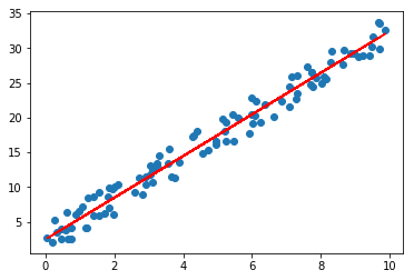
You can see that algorithm learned to draw the most optimal line over the data distribution.
Prediction
Here comes the easy part. Now we have a model with learned parameters which can be used to predict. We can use our hypothesis function.
y = h(3, theta1, theta2)
11.517690816184686
Scikit Learn
Scikit Learn is a python library with one of the most used classical machine learning algorithms. Now you know the what’s happens under the hood of linear regression function. So you are ready to use a library to do production level linear regression machine learning.
Here’s how you import the library
from sklearn.linear_model import LinearRegression
model = LinearRegression()
model.fit(x, y)
fit() function train the data.
model.predict(3)
11.51769082
You can see that values are similar to our own implementation.
Github repo of example code is available here